Traitement des signaux audio de musique -- debruitage: suppression du bruit de fond (De-hissing)
Contents
Introduction: utilisation de LTFAT et preparation
Demarrage de la toolbox ltfat
clear 'variables'; close all; clc;
ltfatstart;
LTFAT version 2.1.1. Copyright 2005-2015 Peter L. S��ndergaard. For help, please type "ltfathelp". LTFAT is using the MEX backend.
(Your global and persistent variables have just been cleared. Sorry.)
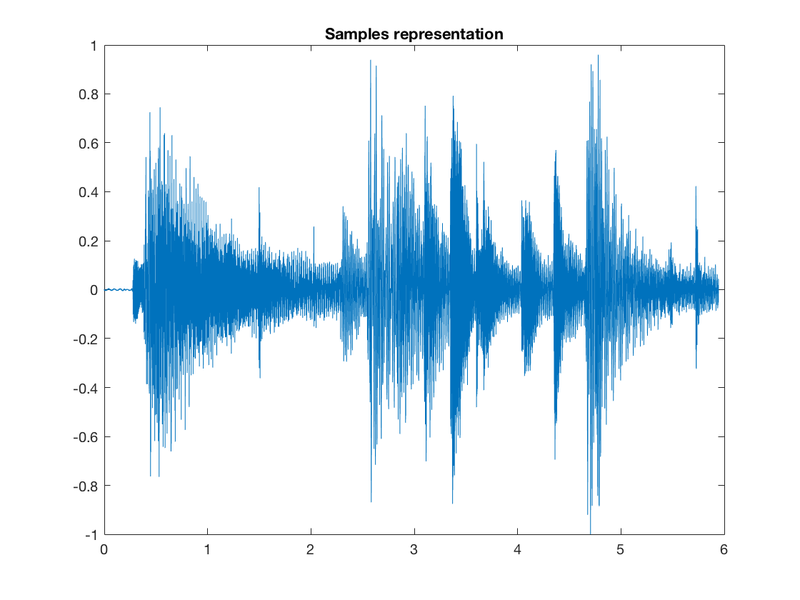
%Lire le fichier audio jazz.wav fourni, ou celui de votre choixa l'aide de
%la fonction audioread, puis l'afficher avec une echelle temporelle adaptee

[x,fs] = audioread('./jazz.wav');
x = x(:);
T = length(x);
TimeAxis = linspace(0,T/fs,T);
figure;
plot(TimeAxis,x);
title('Samples representation');
On s'appuiera sur la toolbox LTFAT pour toutes les transformees temps-frequence. En particulier, on utilisera les fonctions dgtreal} et idgtreal:
help dgtreal
help idgtreal
 DGTREAL  Discrete Gabor transform for real-valued signals
    Usage:  c=dgtreal(f,g,a,M);
            c=dgtreal(f,g,a,M,L);
            [c,Ls]=dgtreal(f,g,a,M);
            [c,Ls]=dgtreal(f,g,a,M,L);

    Input parameters:
          f     : Input data
          g     : Window function.
          a     : Length of time shift.
          M     : Number of modulations.
          L     : Length of transform to do.
    Output parameters:
          c     : M*N array of coefficients.
          Ls    : Length of input signal.

    DGTREAL(f,g,a,M) computes the Gabor coefficients (also known as a
    windowed Fourier transform) of the real-valued input signal f with
    respect to the real-valued window g and parameters a and M. The
    output is a vector/matrix in a rectangular layout.

    As opposed to DGT only the coefficients of the positive frequencies
    of the output are returned. DGTREAL will refuse to work for complex
    valued input signals.

    The length of the transform will be the smallest multiple of a and M*
    that is larger than the signal. f will be zero-extended to the length of
    the transform. If f is a matrix, the transformation is applied to each
    column. The length of the transform done can be obtained by
    L=size(c,2)*a.

    The window g may be a vector of numerical values, a text string or a
    cell array. See the help of GABWIN for more details.

    DGTREAL(f,g,a,M,L) computes the Gabor coefficients as above, but does
    a transform of length L. f will be cut or zero-extended to length L before
    the transform is done.

    [c,Ls]=DGTREAL(f,g,a,M) or [c,Ls]=DGTREAL(f,g,a,M,L) additionally
    returns the length of the input signal f. This is handy for
    reconstruction:

      [c,Ls]=dgtreal(f,g,a,M);
      fr=idgtreal(c,gd,a,M,Ls);

    will reconstruct the signal f no matter what the length of f is, provided
    that gd is a dual window of g.

    [c,Ls,g]=DGTREAL(...) additionally outputs the window used in the
    transform. This is useful if the window was generated from a description
    in a string or cell array.

    See the help on DGT for the definition of the discrete Gabor
    transform. This routine will return the coefficients for channel
    frequencies from 0 to floor(M/2).

    DGTREAL takes the following flags at the end of the line of input
    arguments:

      'freqinv'  Compute a DGTREAL using a frequency-invariant phase. This
                 is the default convention described in the help for DGT.

      'timeinv'  Compute a DGTREAL using a time-invariant phase. This
                 convention is typically used in filter bank algorithms.

    DGTREAL can be used to manually compute a spectrogram, if you
    want full control over the parameters and want to capture the output
    :

      f=greasy;  % Input test signal
      fs=16000;  % The sampling rate of this particular test signal
      a=10;      % Downsampling factor in time
      M=200;     % Total number of channels, only 101 will be computed

      % Compute the coefficients using a 20 ms long Hann window
      c=dgtreal(f,{'hann',0.02*fs'},a,M);

      % Visualize the coefficients as a spectrogram
      dynrange=90; % 90 dB dynamical range for the plotting
      plotdgtreal(c,a,M,fs,dynrange);

    See also:  dgt, idgtreal, gabwin, dwilt, gabtight, plotdgtreal

    References:
      K. Gr��chenig. Foundations of Time-Frequency Analysis. Birkh��user, 2001.

      H. G. Feichtinger and T. Strohmer, editors. Gabor Analysis and
      Algorithms. Birkh��user, Boston, 1998.


    Url: http://ltfat.github.io/doc/gabor/dgtreal.html

 IDGTREAL  Inverse discrete Gabor transform for real-valued signals
    Usage:  f=idgtreal(c,g,a,M);
            f=idgtreal(c,g,a,M,Ls);

    Input parameters:
          c     : Array of coefficients.
          g     : Window function.
          a     : Length of time shift.
          M     : Number of channels.
          Ls    : length of signal.
    Output parameters:
          f     : Signal.

    IDGTREAL(c,g,a,M) computes the Gabor expansion of the input coefficients
    c with respect to the real-valued window g, time shift a and number of
    channels M. c is assumed to be the positive frequencies of the Gabor
    expansion of a real-valued signal.

    It must hold that size(c,1)==floor(M/2)+1. Note that since the
    correct number of channels cannot be deduced from the input, IDGTREAL
    takes an additional parameter as opposed to IDGT.

    The window g may be a vector of numerical values, a text string or a
    cell array. See the help of GABWIN for more details.

    IDGTREAL(c,g,a,M,Ls) does as above but cuts or extends f to length Ls.

    [f,g]=IDGTREAL(...) additionally outputs the window used in the
    transform. This is usefull if the window was generated from a description
    in a string or cell array.

    For perfect reconstruction, the window used must be a dual window of the
    one used to generate the coefficients.

    If g is a row vector, then the output will also be a row vector. If c is
    3-dimensional, then IDGTREAL will return a matrix consisting of one column
    vector for each of the TF-planes in c.

    See the help on IDGT for the precise definition of the inverse Gabor
    transform.

    IDGTREAL takes the following flags at the end of the line of input
    arguments:

      'freqinv'  Use a frequency-invariant phase. This is the default
                 convention described in the help for DGT.

      'timeinv'  Use a time-invariant phase. This convention is typically
                 used in filter bank algorithms.

    Examples:
    ---------

    The following example demostrates the basic pricinples for getting
    perfect reconstruction (short version):

      f=greasy;            % test signal
      a=32;                % time shift
      M=64;                % frequency shift
      gs={'blackman',128}; % synthesis window
      ga={'dual',gs};      %  analysis window

      [c,Ls]=dgtreal(f,ga,a,M); % analysis

      % ... do interesting stuff to c at this point ...

      r=idgtreal(c,gs,a,M,Ls); % synthesis

      norm(f-r)                % test

    The following example does the same as the previous one, with an
    explicit construction of the analysis and synthesis windows:

      f=greasy;     % test signal
      a=32;         % time shift
      M=64;         % frequency shift
      Ls=length(f); % signal length

      % Length of transform to do
      L=dgtlength(Ls,a,M);

      % Analysis and synthesis window
      gs=firwin('blackman',128);
      ga=gabdual(gs,a,M,L);

      c=dgtreal(f,ga,a,M);  % analysis

      % ... do interesting stuff to c at this point ...

      r=idgtreal(c,gs,a,M,Ls); % synthesis

      norm(f-r)       % test

    See also:  idgt, gabwin, gabdual, dwilt

    Url: http://ltfat.github.io/doc/gabor/idgtreal.html
il pourra etre utile d'utiliser les "pointeurs de fonctions" matlab, qui permettent de simplifier le code. En pratique, cela evitera de passer tous les parametres necessaires de dgtreal a une fonction: on passera simplement le nom de la fonction qui l'encapsule. Par exemple, on cree une fonction {\tt op.analysis} qui permet d'implementer l'operateur d'analyse d'une transformee de Gabor avec une fenetre de Hann
%M de taille 1024, avec 50\% de recouvrement:

M = 1024;
a = M/4;
T = length(x);
g = gabwin({'tight', 'hann'}, a, M);

op.analysis = @(x) dgtreal(x,g,a,M);
op.synthesis = @(x) idgtreal(x,g,a,M,T);
Ainsi, il suffit d'appeler op.analysis(x) pour faire l'analyse temps-frequence du signal x
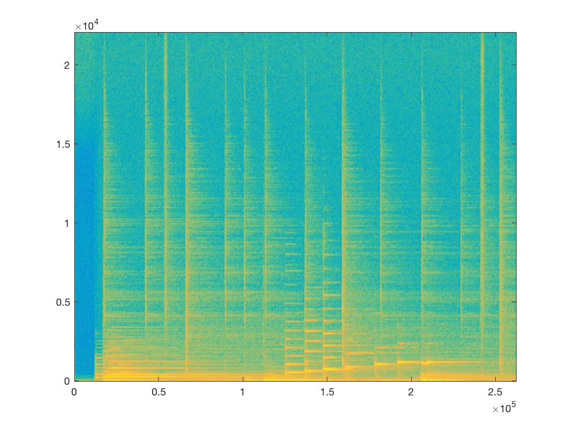
X = op.analysis(x);
[NbFreq, NbTime] = size(X);
FreqGaborAxis = linspace(0,fs/2,NbFreq);
TimeGaborAxis = linspace(0,T,NbTime);
figure;
imagesc(TimeGaborAxis, FreqGaborAxis, 20*log(abs(X)+eps));
set(gca,'Ydir','Normal');
et op.synthesis pour faire la synthese:
x_reconstruit = op.synthesis(X);
err = norm(x(:)-x_reconstruit(:))^2;
fprintf('erreur de reconstruction: %f\n',err);
erreur de reconstruction: 0.000000
Dans une fonction, on pourra passer simplement la variable op pour beneficier de op.analysis et op.synthesis. Exemple:
function [X,x_rec] = func_ex(x,op)
   T = length(x);
   X = op.analysis(x);
   x_rec = op.synthesis(X);
 end
[X, x_rec] = func_ex(x,op);

[NbFreq, NbTime] = size(X);
FreqGaborAxis = linspace(0,fs/2,NbFreq);
TimeGaborAxis = linspace(0,T,NbTime);
figure;
imagesc(TimeGaborAxis, FreqGaborAxis, 20*log(abs(X)+eps));
set(gca,'Ydir','Normal');

err = norm(x(:)-x_rec(:))^2;
fprintf('erreur de reconstruction: %f\n',err);
erreur de reconstruction: 0.000000

Generation de bruits blanc ou colores et estimation spectrale
La fonction noise_gen permet de generer un bruit blanc ou colore
help noise_gen

noise_type = 'white';
[noise,spectrum] = noise_gen(T,1,fs,noise_type);
  NOISE  Stochastic noise generator
    Usage: outsig = noise(siglen,nsigs,type);

    Input parameters:
        siglen    : Length of the noise (samples)
        nsigs     : Number of signals (default is 1)
        type      : type of noise. See below.

    Output parameters:
        outsig    : siglen xnsigs signal vector

    NOISE(siglen,nsigs) generates nsigs channels containing white noise
    of the given type with the length of siglen. The signals are arranged as
    columns in the output. If only siglen is given, a column vector is
    returned.

    NOISE takes the following optional parameters:

      'white'  Generate white (gaussian) noise. This is the default.

      'pink'   Generate pink noise.

      'brown'  Generate brown noise.

      'red'    This is the same as brown noise.

    By default, the noise is normalized to have a unit energy, but this can
    be changed by passing a flag to NORMALIZE.

    Examples:
    ---------

    White noise in the time-frequency domain:

      sgram(noise(5000,'white'),'dynrange',70);

    Pink noise in the time-frequency domain:

      sgram(noise(5000,'pink'),'dynrange',70);

    Brown/red noise in the time-frequency domain:

      sgram(noise(5000,'brown'),'dynrange',70);

    See also: normalize

    Url: http://ltfat.sourceforge.net/doc/signals/noise.php
La methode de Welch permet d'estimer la densite spectrale de puissance du bruit. Pour cela, il suffit de faire la transformer de Gabor du bruit, puis de moyenner les densit?s spectrales obtenues dans chaque fenetre
Exercice 1: implementer l'estimateur de Welch
[dsp_noise] = welch(noise,op,g)
Entrees:
  - noise: le vecteur contenant le bruit
  - op:    l'operateur permettant de faire l'analyse de Gabor voulue
  - g:     fenetre d'analyse utilisee dans l'operateur (necessaire pour normalisation)
Sortie:
  - dsp_nosise: l'estimation de la densite spectrale de puissance du bruit
[dsp_noise] = welch(noise,op,g);
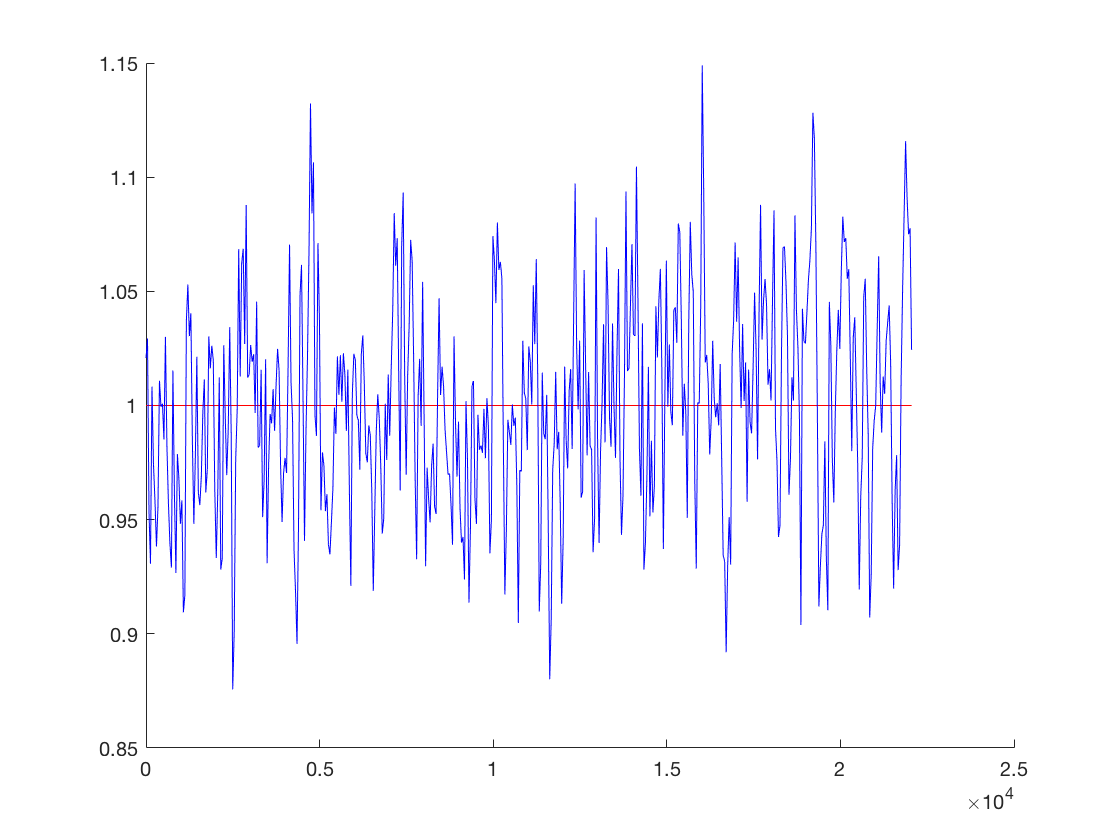
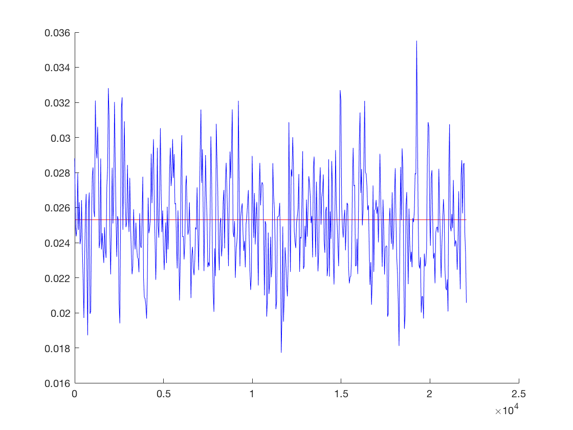
On compare la dsp estimee et la dsp theorique
figure;
hold on
FreqAxisTrue = linspace(0,fs/2,length(spectrum));
plot(FreqAxisTrue,spectrum,'r');
FreqAxisEstim = linspace(0,fs/2,length(dsp_noise));
plot(FreqAxisEstim,dsp_noise,'b');
hold off
On va maintenant simuler l'ajout d'un bruit de fond. La fonction noise_gen generant un bruit de variance 1, on va ajuster l'energie de bruit pour atteindre un SNR en entree fixee
Input_SNR = 0 ;
sigma_bruit = sqrt(var(x)*10^(-Input_SNR/10));

noise = sigma_bruit*noise;
y = x + noise;
On verifie le SNR en entree:
fprintf('Input SNR = %f\n',SNR(x,y));
Input SNR = 0.000004
On va simuler l'hypothese: on observe une partie du signal qui ne contient que du bruit sur 1 s, qui permet d'estimer la dsp du bruit
Tnoise = fs;

noiseObserved = noise(1:Tnoise);
[dsp_noise] = welch(noiseObserved,op,g);
figure;
hold on
FreqAxisTrue = linspace(0,fs/2,length(spectrum));
plot(FreqAxisTrue,sigma_bruit^2*spectrum,'r');
FreqAxisEstim = linspace(0,fs/2,length(dsp_noise));
plot(FreqAxisEstim,dsp_noise,'b');
hold off
Debruitage par estimation diagonale
La premiere methode vue est le filtrage "a la Wiener" empirique, sans parametre
Y = op.analysis(y);

HWienerNum = bsxfun(@minus,abs(Y).^2,dsp_noise); %Noter l'utilisation de bsxfun + dspNoise est deja une puissance
HWienerNum(HWienerNum < 0) = 0;
HWienerDenum = abs(Y).^2;


HWiener = HWienerNum./(HWienerDenum+eps); % +eps pour eviter les divisions par 0
X_estim = Y.*HWiener ;

x_estim = op.synthesis(X_estim);
On evalue le SNR en sortie
Output_SNR = SNR(x,x_estim);

fprintf('Output SNR = %f\n',Output_SNR);
Output SNR = 12.903996
Exercice 2: implementer une methode generale de debruitage, permettant d'effectuer Wiener empirique ou soustraction spectrale, avec plusieurs parametres. On pourra fixer certains parametres par defaut
[x_denoise] = DeHiss(x,noise,op,lambda,alpha,beta,gamma)
De Hissing par estimation diagonale dans le domaine T.F.
    XDenoise = X .* H
avec
    H = max(gamma x DspN ;
             (|X|alpha-lambda|DspN|^(alpha/2))./|X|^alpha) ) ^ beta)
ou DspN est une estimation de la densit? spectrale de puissance du bruit
Entree:
- x: signal a debruiter
- noise: bruit isole
- op: operateurs d'analyse/synthese
- lambda: valeur du seuillage
- alpha: puissance du module (defaut alpha = 2)
- beta: puissance du filtre (defaut beta = 1)
- gamma: bruit residuel (defaut gamma = 1e-4)
Sortie:
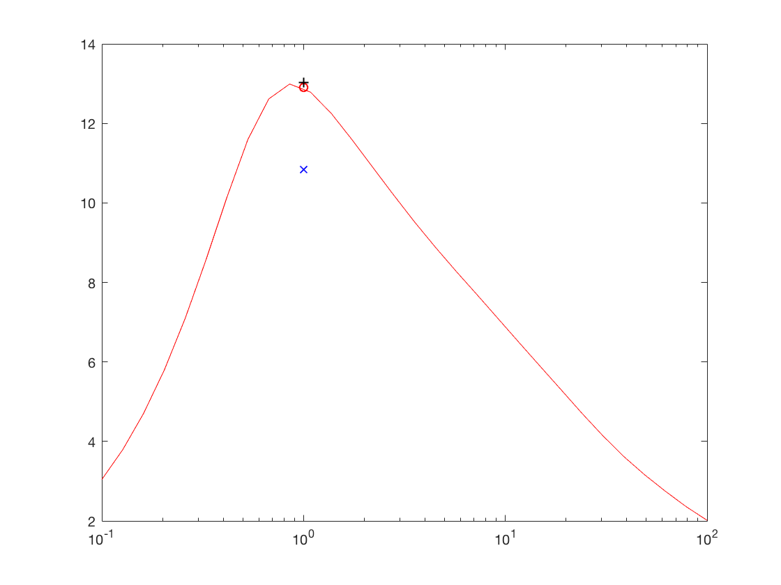
- x_denoise: signal debruiteOn testera cette methode avec les valeurs par defaut pour commencer, en faisant varier le parametre lambda.
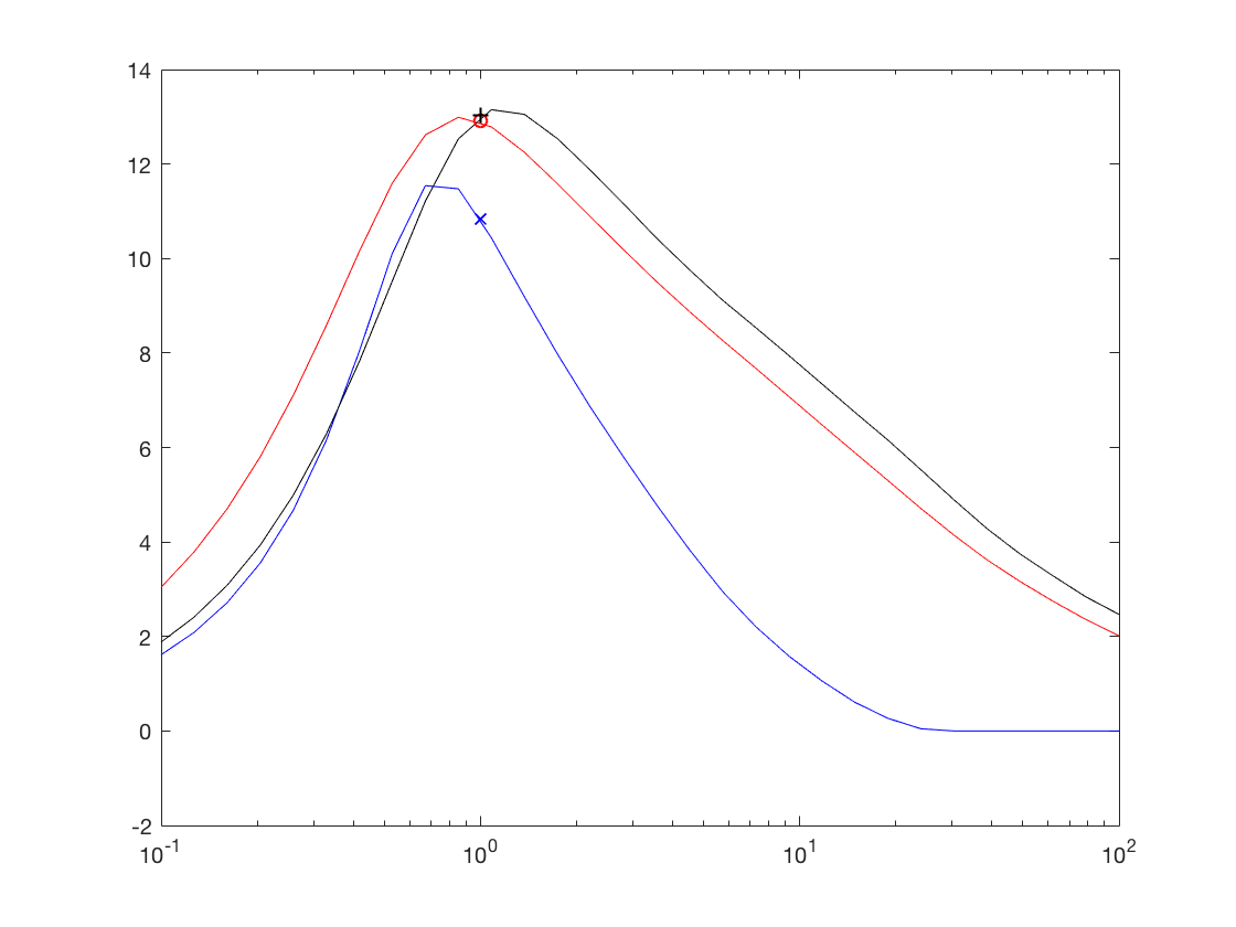
Enfin, on dessinera la courbe SNR en sortie VS lambda. On choisira une echelle logarithmique pour les lambda
faire apparaitre sur cette courbe les resultats obtenus par le Wiener Empirique sans ponderation par lambda
Exo2
Exercice 3: reprendre l'exercice precedent, en supperposant les courbes obtenues pour differents gamma = [1e-1,1e-2,..,1e-6,0]
Exo3
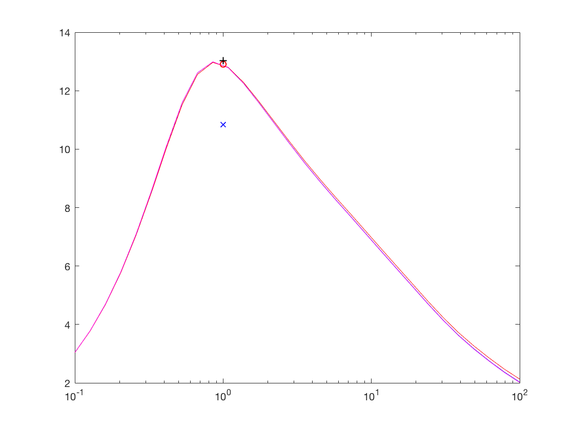
Exercice 4: comparer les courbes pour differents gamma = [1e-1,1e-2,..,1e-6,0] , beta = [1,2] et alpha = [1,2] . dessiner les cources pour le meilleur gamma, et faire apparaitre les resultats obtenus pour le Wiener Empirique, la soustraction spectrale d'amplitude et la soustraction spectrale de puissance ( lambda = 1 )
Exo4