Audio denoising by (iterative) thresholding

Preliminaries
Simple thresholding in TF domain
Structured thresholding with WG-LASSO
Iterative thresholding
Tonal + Transient + Noise Hybrid decomposition

Preliminaries

Download the Linear Time-Frequency Analysis Toolbox (LTFAT) on http://ltfat.sourceforge.net Add the ltfat TB directory to MatLab Path and check that the installation is correct

ltfatstart

Warning: BLOCKPROCINIT: JVM support not present. 
LTFAT version 2.1.1. Copyright 2005-2015 Peter L. SÃ¸ndergaard. For help, please type "ltfathelp". LTFAT is using the MEX backend.
(Your global and persistent variables have just been cleared. Sorry.)

LTFAT is curently using the matlab backend. To speed it up, we will compile the mexfiles

ltfatmex

========= Compiling libltfat ==============
Done.
========= Compiling MEX interfaces ========
   ...using libmwfftw3.3.dylib from Matlab installation.
   ...using libmwfftw3f.3.dylib from Matlab installation.
Done.
========= Compiling GPC ===================
Done.

Clear everything and re-start ltfat. Now LTFAT should use the mex backend

clc;close all;clear all;
ltfatstart;

Warning: BLOCKPROCINIT: JVM support not present. 
LTFAT version 2.1.1. Copyright 2005-2015 Peter L. SÃ¸ndergaard. For help, please type "ltfathelp". LTFAT is using the MEX backend.
(Your global and persistent variables have just been cleared. Sorry.)

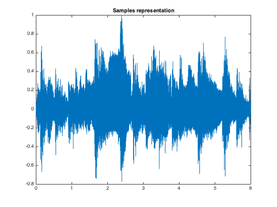
Load the signal and display its time samples

[s,Fs]  = audioread('quintet.wav');

T = length(s);
Time = linspace(0,T/Fs,T);

figure;
plot(Time, s);
title('Samples representation');

choose the input snr and add some noise

snr_level = 10;
sigma_noise = norm(s)^2*10^(-snr_level/10)/T;
noise = sqrt(sigma_noise)*randn(size(s));

xn = s + noise;

%Check the input snr
disp(snr(s,xn));

   10.0004

Simple thresholding in TF domain

Set the Gabor parameters: window length and shape and overlap. Here, we use a 1024 samples (tight) Hann window, with 50% overlap.

M = 1024;
a = M/2;
g = gabwin({'tight', 'hann'}, a, M);

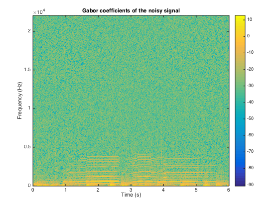
Gabor transform of the noisy signal and display it

G_xn = dgtreal(xn, g, a, M);
figure;
plotdgtreal(G_xn,a,M,Fs);
title('Gabor coefficients of the noisy signal');

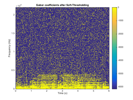
Performs soft thresholding with a fixed \lambda. We choose \lambda=\sigma as spectral substraction suggests.

lambda = sqrt(sigma_noise);
G_xd = G_xn.*max(0,1-lambda./abs(G_xn));
figure;
plotdgtreal(G_xd,a,M,Fs);
title('Gabor coefficients after Soft-Thresholding');

Compute the resulting output SNR

xd = idgtreal(G_xd,g,a,M,T);
disp(snr(s,xd));

   16.3585

Structured thresholding with WG-LASSO

We firt create the "sliding" window used to define the neighborhood. We choose a neighborhood with two coefficients before and after on the time axis

K = 5; %total size of the neighborhood
neigh = ones(1,K);
neigh = neigh/norm(neigh(:),1);

% We define the center of the window
c = ceil(K/2);

We must create a matrix to stock the local energy of each neighborhood. To deal with the right and left edges, where the coefficients are mirrowed

We create make a larger matrix with mirrowed borders and put the gabor squared coefficients in the middle

[MG,NG] = size(G_xn);% stock the usefull sizes
W = zeros(MG, NG+K-1);
W(:, c: NG+c-1) = abs(G_xd).^2;
W(:, 1:c-1) =  fliplr(W(:, c : 2*(c-1))); % left border
W(:, NG+c:end) = fliplr(W(:, NG - K +2*c: NG+c-1));% right border

finaly, compute the neighborhood energy thanks to a convolution and resize the matrix

W = (conv2(W, neigh, 'same'));
W = W(:, c : NG + c -1);

take the square root to obtain the norm of the neighborhood, and perform threhsolding

W = sqrt(W);
G_xd = G_xn.*max(0,1-(lambda./W));

figure;
plotdgtreal(G_xd,a,M,Fs);
title('Gabor coeff. after WGLASSO thresholding');

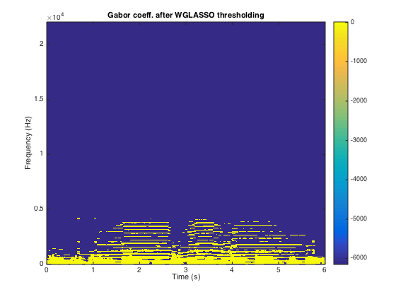
Compute the resulting output SNR

xd = idgtreal(G_xd,g,a,M,T);
disp(snr(s,xd));

   14.5880

One can remarks that the time-frequency coefficients are much more structured. However, with the same value of \lambda=\sigma, the output SNR is better with Soft Thresholding. We will now compare the results for various value of \lambda.

Exercice 1 : a denoising is performed by soft thresholding or wg-lasso of the gabor coefficients of the noisy signal. Compute the denoising SNR with both thresholding. Spot the threshold that gives a residual with a variance close to the variance of the noise

exo1;

Iterative thresholding

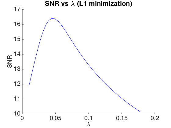
We now will perform the true L1 minimization, instead of one simple SoftThresholding step.

Firt, set up the parameters (number of iterations etc.) and create the vectors to stock the results

nbit = 30; %number of iteration for ISTA
nb_xp = 30; % number of values for the parameter
lambda_values_it = logspace(-3/4,-2,nb_xp);%generate the vector of parameter


snr_soft_it = zeros(nb_xp,1);
sigma_soft_it = zeros(nb_xp,1);

We intialise the algorithm with 0

G_xd = 0.*G_xn;
k=0;

and run ISTA for various lambda

for lambda=lambda_values_it
    k = k+1; % XP number k
    for it=1:nbit % ISTA loop
        r = xn-idgtreal(G_xd,g,a,M,T);
        G_xd = G_xd + dgtreal(r, g, a, M); % Gradient step
        G_xd = G_xd.*max(0,1-lambda./abs(G_xd)); % Thresholding step
    end
    xd_soft = idgtreal(G_xd,g,a,M,T); % Back to the time domain
    sigma_soft_it(k) = var(xn-xd_soft); % Compute the variance of the residual
    snr_soft_it(k) = snr(s,xd_soft); % Compute the output SNR
end

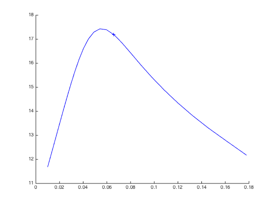
Plot the results

figure;
hold on
plot(lambda_values_it,snr_soft_it,'b');
[~,k_soft] = min(abs(sigma_soft_it-sigma_noise));
plot(lambda_values_it(k_soft),snr_soft_it(k_soft),'+b');
set_graphic_sizes([], 20,2);
set_label('\lambda', 'SNR');
title('SNR vs \lambda (L1 minimization)')
hold off

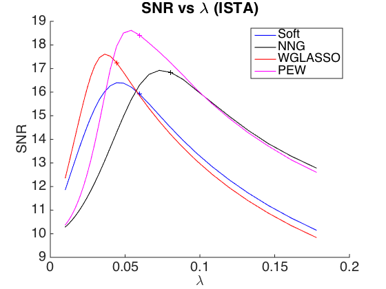
As with simple thresholding, we can can use various thresholding operator in ISTA.

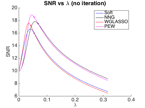
Exercice 2 : compare the denoising effect with ISTA and various thresholding operator (soft, Kg, wg-lasso, PEW...). Plot the SNR VS the parameter and spot the parameter giving a residual with a variance close to the variance of the noise

exo2;

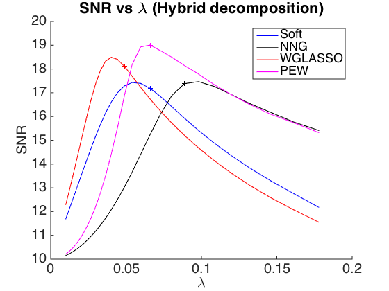
Tonal + Transient + Noise Hybrid decomposition

Set the gabors parameters for transient (short Hann window with 50% overlap)

M1 = 64;
a1 = M1/2;
g1 = gabwin({'tight', 'hann'}, a1, M1);
G_xn1 = dgtreal(xn, g1, a1, M1);

and for tonal (long Hann window with 50% overlap)

M2 = 4096;
a2 = M2/2;
g2 = gabwin({'tight', 'hann'}, a2, M2);

G_xn2 = dgtreal(xn, g2, a2, M2);

Set the number of iteration for ISTA and the number of lambda parameter

nbit = 30;
nb_xp = 30;
lambda_values_double = logspace(-3/4,-2,nb_xp);

ton+trans+noise hybrid decomposition with ISTA and Soft thresholding

snr_soft_double = zeros(nb_xp,1);
sigma_soft_double = zeros(nb_xp,1);


G_xd1 = 0.*G_xn1;
G_xd2 = 0.*G_xn2;

k=0;
for lambda=lambda_values_double
    k = k+1;
    for it=1:nbit
        G_xd_old1 = G_xd1;
        G_xd_old2 = G_xd2;

        r = xn-idgtreal(G_xd1,g1,a1,M1,T)-idgtreal(G_xd2,g2,a2,M2,T);
        G_xd1 = G_xd1 + dgtreal(r, g1, a1, M1)/2;
        G_xd2 = G_xd2 + dgtreal(r, g2, a2, M2)/2;

        G_xd1 = G_xd1.*max(0,1-(lambda/2)./abs(G_xd1));
        G_xd2 = G_xd2.*max(0,1-(lambda/2)./abs(G_xd2));
    end
    xd_trans = idgtreal(G_xd1,g1,a1,M1,T);
    xd_ton = idgtreal(G_xd2,g2,a2,M2,T);
    xd_soft =  xd_trans + xd_ton;

    sigma_soft_double(k) = var(xn-xd_soft);
    snr_soft_double(k) = snr(s,xd_soft);
end

plot the results

figure;
hold on
plot(lambda_values_double,snr_soft_double,'b');
[~,k_soft] = min(abs(sigma_soft_double-sigma_noise));
plot(lambda_values_double(k_soft),snr_soft_double(k_soft),'+b');
hold off

Exercice 3 : compare the denoising effect with the decompoistion ton+trans+noise and various thresholding (soft, Kg, wg-lasso, PEW...).

For WG-Lasso, you can use a neighborhood for the transients with 2 coefficients before and after along the Frequency axis.

Plot the SNR VS the parameter and spot the parameter giving a residual with a variance close to the variance of the noise